Benchmarking every backend

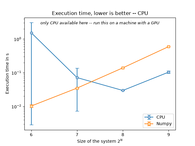
Every backend available here against a hand-rolled numpy split step, over a range of grid sizes.

Benchmarks:   0%|          | 0/16 [00:00<?, ?it/s]
Benchmarks:   6%|▋         | 1/16 [00:03<00:46,  3.07s/it]
Benchmarks:  31%|███▏      | 5/16 [00:03<00:05,  2.04it/s]
Benchmarks:  56%|█████▋    | 9/16 [00:03<00:01,  4.23it/s]
Benchmarks:  75%|███████▌  | 12/16 [00:03<00:00,  5.34it/s]
Benchmarks:  88%|████████▊ | 14/16 [00:03<00:00,  6.02it/s]
Benchmarks: 100%|██████████| 16/16 [00:05<00:00,  3.54it/s]
Benchmarks: 100%|██████████| 16/16 [00:05<00:00,  3.17it/s]

import os
import time

import matplotlib.pyplot as plt
import numpy as np
import tqdm
from _output import output_path
from cycler import cycler
from NLSE import NLSE
from NLSE.backends import list_available_backends

# Propagation step, passed to out_field and used by the plots below.
DELTA_Z = 1e-4

# for plots
tab_colors = [
    "tab:blue",
    "tab:orange",
    "forestgreen",
    "tab:red",
    "tab:purple",
    "tab:brown",
    "tab:pink",
    "tab:gray",
    "tab:olive",
    "teal",
]
fills = [
    "lightsteelblue",
    "navajowhite",
    "darkseagreen",
    "lightcoral",
    "violet",
    "indianred",
    "lavenderblush",
    "lightgray",
    "darkkhaki",
    "darkturquoise",
]
edges = tab_colors
custom_cycler = (
    (cycler(color=tab_colors))
    + (cycler(markeredgecolor=edges))
    + (cycler(markerfacecolor=fills))
)
plt.rc("axes", prop_cycle=custom_cycler)

PRECISION = "lie"
if PRECISION == "strang":
    PRECISION_REAL = np.float64
    PRECISION_COMPLEX = np.complex128
else:
    PRECISION_REAL = np.float32
    PRECISION_COMPLEX = np.complex64

n2 = -1.99e-9
n12 = -0.75e-10
waist = 2.29e-3
waist_d = 70e-6
nl_length = 0
d_real = 3.76e-6
d_fourier = 5.5e-6
f_fourier = 200e-3
window = 3008 * d_real
puiss = 1.05
Isat = 3.92e4  # saturation intensity in W/m^2
L = 2e-3
alpha = 22
dn = None
N_avg = 2
# A documentation build sets NLSE_DOCS_BUILD and gets the small sweep, so the
# gallery shows a real graph made by this script rather than a placeholder.
# Run it yourself and you get the full range.
sizes = (
    np.logspace(6, 9, 4, base=2, dtype=int)
    if os.environ.get("NLSE_DOCS_BUILD")
    else np.logspace(6, 14, 9, base=2, dtype=int)
)
# One column per backend that exists here, plus the hand-rolled numpy
# split step as the thing they are all being compared against. It used
# to ask for "CUPY" by name, which on a machine without it falls back to
# the CPU and draws two CPU curves under different labels.
BACKENDS = list_available_backends()
times = np.zeros((len(sizes), len(BACKENDS) + 1, N_avg))
pbar = tqdm.tqdm(total=np.prod(times.shape), desc="Benchmarks")
for i, size in enumerate(sizes):
    for j, backend in enumerate(BACKENDS):
        simu0 = NLSE(
            alpha,
            puiss,
            window,
            n2,
            None,
            L,
            NX=size,
            NY=size,
            nl_length=nl_length,
            backend=backend,
        )
        simu0.I_sat = Isat
        if j == 0:
            E_0 = np.exp(-(np.hypot(simu0.XX, simu0.YY) ** 2) / waist**2).astype(
                PRECISION_COMPLEX
            )
        for k in range(N_avg):
            t0 = time.perf_counter()
            simu0.out_field(E_0, L, verbose=False, delta_z=DELTA_Z)
            times[i, j, k] = time.perf_counter() - t0
            pbar.update(1)
    # numpy naive implementation
    for k in range(N_avg):
        E1 = E_0.copy()
        t0 = time.perf_counter()
        for _ in range(int(L / DELTA_Z)):
            E1 = np.fft.fft2(E1)
            E1 *= np.exp(1j * DELTA_Z * simu0.propagator / (2 * simu0.k))
            E1 = np.fft.ifft2(E1)
            E1 *= np.exp(
                1j
                * DELTA_Z
                * simu0.k
                * simu0.n2
                * np.abs(E1) ** 2
                / (1 + np.abs(E1) ** 2 / Isat)
            )
            E1 *= np.exp(-simu0.alpha * DELTA_Z)
        times[i, len(BACKENDS), k] = time.perf_counter() - t0
        pbar.update(1)
pbar.close()
np.save(output_path("benchmarks_times.npy"), times)
np.save(output_path("benchmarks_sizes.npy"), sizes)
fig, ax = plt.subplots()
MARKERS = ["o", "s", "^", "v", "D"]
for j, label in enumerate([*BACKENDS, "Numpy"]):
    mean = np.mean(times[:, j, :], axis=-1)
    ax.errorbar(
        np.log2(sizes).astype(int),
        mean,
        yerr=[
            mean - np.min(times[:, j, :], axis=-1),
            np.max(times[:, j, :], axis=-1) - mean,
        ],
        label=label,
        marker=MARKERS[j % len(MARKERS)],
        capsize=4,
    )
ax.legend()
ax.set_xticks(np.log2(sizes).astype(int))
ax.set_xlabel(r"Size of the system $2^N$")
ax.set_ylabel("Execution time in s")
ax.set_title(f"Execution time, lower is better -- {', '.join(BACKENDS)}")
# A backend comparison is only a comparison if there is more than one backend.
# The documentation runner has no GPU and no OpenCL, so the figure published
# with these docs has a single bar; say so on it rather than let a reader take
# CPU-only for the whole story.
if len(BACKENDS) == 1:
    ax.text(
        0.5,
        0.94,
        f"only {BACKENDS[0]} available here -- run this on a machine with a GPU",
        transform=ax.transAxes,
        ha="center",
        fontsize=9,
        style="italic",
    )
ax.set_yscale("log")
fig.savefig(output_path("benchmarks.svg"), dpi=300)
plt.show()