Jones-Roberts solitons

The soliton family of a 2D superfluid, and the trip along it, after Baker-Rasooli et al., Phys. Rev. Lett. 134, 233401 (2025).

A one-dimensional fluid has dark solitons. A two-dimensional one has a whole family of solitary waves, found by Jones and Roberts in 1982, and the family has two halves: a vortex pair at low speed, a rarefaction pulse – a density dip carrying no circulation at all – at high speed, and a critical speed where one becomes the other. What makes it a family rather than two unrelated objects is that a single soliton can travel along it.

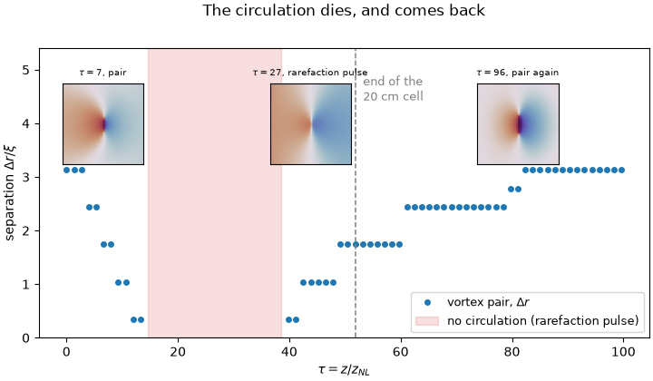
That is what this page shows, in a single propagation. Two counter-rotating circulations are imprinted on the beam, as the experiment imprints them with a spatial light modulator, and left alone. They drift together; the depletion between them fills in; and the two phase singularities meet and annihilate, leaving behind a rarefaction pulse – a solitary wave that still travels, still holds together, and has no circulation anywhere in it. Nothing is done to it in between. The soliton walks from one half of the family into the other on its own.

The parameters are the experiment’s, from the paper’s supplementary material: 5 W in a 2.23 mm waist through 20 cm of rubidium at 150 °C, 780 nm and about -10 GHz detuned, \(n_2 = -1.04\times10^{-10}\,\mathrm{m^2/W}\), \(I_{sat} = 60\,\mathrm{W/cm^2}\), and the ~30% losses the paper quotes. Two checks that they are the right ones: they put the beam at 71 healing lengths across, against the fluid radius of \(63\,\xi\) the paper states, and they put the 20 cm cell at \(\tau = 52\), against the \(\tau > 52\) the paper gives for the onset of the transition – the cell ends just about where the circulation dies.

The experiment reaches other \(\tau\) by scanning the fluid beam power, since its cell has one length. A simulation has the whole propagation in hand, so this one simply runs on past the cell to \(\tau = 100\) and watches.

Note

Two conventions travel with this paper and neither is the Bogoliubov one. Its nonlinear length is \(z_{NL} = 1/k_0\Delta n\) and its healing length \(\xi = \sqrt{z_{NL}/k_0}\), both built from \(\Delta n\) rather than from \(c_s^2 = I\,\partial\Delta n/\partial I\). In a saturable medium those differ by \(\sqrt{1+I/I_{sat}}\), which is 1.44 here – 21.9 µm against 31.4 µm. The paper’s are used throughout, so that \(\tau\) and \(\Delta r/\xi\) mean what they mean in the paper.

Warning

The step size for a run like this is a stability condition, not an accuracy one. Split-step applies the linear part exactly in Fourier space, so dispersion cannot limit accuracy on its own – but on a finite-amplitude background the nonlinear step couples modes, and past about a radian of linear phase per step at the grid’s highest wavenumber the resonant modes grow out of round-off. It does not look numerical when it happens: the background fills with density fluctuations of order the density itself and thousands of spurious vortices, which reads as the fluid going turbulent. The solver enforces the bound itself and warns when it reduces the step.

import matplotlib.pyplot as plt
import numpy as np
from matplotlib.animation import FuncAnimation
from NLSE import NLSE
from scipy.integrate import solve_ivp
from scipy.optimize import brentq

The experiment’s parameters, from the supplementary material.

N2 = -1.04e-10  # nonlinear index in m^2/W, defocusing
I_SAT = 60e4  # saturation intensity, 60 W/cm^2
POWER = 5.0  # fluid beam power in W
WAIST = 2.23e-3  # fluid beam waist in m
L_CELL = 20e-2  # cell length in m
TRANSMISSION = 0.7  # the paper's ~30% losses
WVL = 780e-9  # 87Rb D2, about -10 GHz detuned, cell at 150 C
N_PTS = 1024

K0 = 2 * np.pi / WVL
I0 = 2 * POWER / (np.pi * WAIST**2)  # peak intensity of the Gaussian
DN = abs(N2) * I0 / (1 + I0 / I_SAT)  # saturated index depression
Z_NL = 1 / (K0 * DN)  # the paper's nonlinear length
XI = np.sqrt(Z_NL / K0)  # the paper's healing length
XI_BOGOLIUBOV = (1 + I0 / I_SAT) / (K0 * np.sqrt(abs(N2) * I0))

# The window holds the beam and the dark surround it decays into. That the
# beam is Gaussian rather than uniform matters for more than realism: the
# intensity falls to nothing at the edges, so the periodic boundary has no
# fluid to join up. A dipole's phase is only periodic to order dr/W, and on a
# uniform background that mismatch radiates from the seam and fringes the
# whole picture.
WINDOW = 3.5 * WAIST
DX = WINDOW / N_PTS

# Past the cell, which is tau = 52 -- where the paper puts the onset of the
# transition -- so the rarefaction pulse can be watched for a while after it
# forms rather than only at the moment it does.
TAU_END = 100
LENGTH = TAU_END * Z_NL

print(
    f"medium: Dn = {DN:.2e}, z_NL = {Z_NL * 1e3:.2f} mm, xi = {XI * 1e6:.1f} um "
    f"(Bogoliubov xi would be {XI_BOGOLIUBOV * 1e6:.1f} um)"
)
print(
    f"beam:   {POWER} W, waist {WAIST * 1e3:.2f} mm = {WAIST / XI:.0f} xi, "
    f"I0 = {I0 / I_SAT:.2f} Isat"
)
print(
    f"cell:   {L_CELL * 1e2:.0f} cm = tau {L_CELL / Z_NL:.0f}; this run goes to "
    f"tau {TAU_END}"
)
print(f"grid:   {N_PTS}^2, dx = xi/{XI / DX:.1f}, window = {WINDOW / XI:.0f} xi")


def small_signal_alpha():
    """Return the alpha whose saturable absorption gives TRANSMISSION.

    The medium bleaches where the beam is bright, so the loss is not
    exponential and ``-log(T)/L`` is not the coefficient to hand the solver.
    Solved on the radial profile instead.

    Returns
    -------
    float
        Small-signal absorption coefficient in 1/m.
    """
    r = np.linspace(0, 3 * WAIST, 800)
    profile = I0 * np.exp(-2 * r**2 / WAIST**2)

    def transmitted(alpha):
        """Power fraction left after the cell at this alpha."""
        solution = solve_ivp(
            lambda z, intensity: -alpha * intensity / (1 + intensity / I_SAT),
            (0, L_CELL),
            profile,
            rtol=1e-9,
            atol=1e-12,
        )
        return np.trapezoid(solution.y[:, -1] * 2 * np.pi * r, r) / np.trapezoid(
            profile * 2 * np.pi * r, r
        )

    return brentq(lambda a: transmitted(a) - TRANSMISSION, 1e-4, 500, xtol=1e-9)


ALPHA = small_signal_alpha()
print(
    f"loss:   alpha = {ALPHA:.2f}/m for {TRANSMISSION:.0%} over the cell "
    f"(a plain exponential would say {-np.log(TRANSMISSION) / L_CELL:.2f})"
)


def vortex(simu, x0, y0, charge):
    """Return one vortex: a phase winding with a healed core.

    Parameters
    ----------
    simu : NLSE
        Solver, for its coordinate grids.
    x0, y0 : float
        Core position in m.
    charge : int
        Sign of the circulation.

    Returns
    -------
    ndarray
        Complex field of unit modulus far from the core.

    Notes
    -----
    The core profile only needs the right asymptotics; whatever is imprinted
    radiates its excess within a few nonlinear lengths and relaxes onto the
    true one. A Pade profile was tried and left no less sound behind, which
    says the relaxation is set by the dipole and not by the core.
    """
    x, y = simu.XX - x0, simu.YY - y0
    r = np.hypot(x, y)
    return r / np.sqrt(r**2 + XI**2) * np.exp(1j * charge * np.arctan2(y, x))


def singularities(field):
    """Return the pixel coordinates of the phase singularities.

    How many there are is what says which half of the family the soliton is
    in: two for a vortex pair, none for a rarefaction pulse.

    Parameters
    ----------
    field : ndarray
        Complex field.

    Returns
    -------
    tuple of ndarray
        Column indices, row indices, and the sign of each circulation.
    """
    phase = np.angle(field)
    dx = np.angle(np.exp(1j * (np.roll(phase, -1, axis=1) - phase)))
    dy = np.angle(np.exp(1j * (np.roll(phase, -1, axis=0) - phase)))
    curl = dx + np.roll(dy, -1, axis=1) - np.roll(dx, -1, axis=0) - dy
    rows, cols = np.where(np.abs(curl) > np.pi)
    return cols, rows, np.sign(curl[rows, cols])

medium: Dn = 3.22e-05, z_NL = 3.85 mm, xi = 21.9 um (Bogoliubov xi would be 31.4 um)
beam:   5.0 W, waist 2.23 mm = 102 xi, I0 = 1.07 Isat
cell:   20 cm = tau 52; this run goes to tau 100
grid:   1024^2, dx = xi/2.9, window = 357 xi
loss:   alpha = 2.52/m for 70% over the cell (a plain exponential would say 1.78)

The imprint, and the propagation. The pair goes in off-centre, as the paper puts it: the Gaussian carries a density gradient, so the healing length the pair sits in changes as it travels, and it is that changing \(\Delta r/\xi\) which walks the soliton along the family.

# Just above the critical separation. Below about 2.5 xi the pair annihilates
# within a couple of nonlinear lengths, which is over before the animation
# starts; above 3 xi it survives the whole run. This sits in between, so the
# transition happens on screen.
SEPARATION = 3.0 * XI
simu = NLSE(
    ALPHA, POWER, WINDOW, N2, None, LENGTH, NX=N_PTS, NY=N_PTS, Isat=I_SAT, wvl=WVL
)
envelope = np.exp(-(simu.XX**2 + simu.YY**2) / WAIST**2)
E_in = (
    envelope
    * vortex(simu, -0.25 * WAIST, +SEPARATION / 2, +1)
    * vortex(simu, -0.25 * WAIST, -SEPARATION / 2, -1)
).astype(np.complex64)

frames, taus, gaps, counts, centres = [], [], [], [], []


def follow(sim, A, z, i):
    """Sample the field, and how far apart the two circulations are."""
    if i % 120:
        return
    field = np.asarray(sim._backend.to_numpy(A))
    cols, rows, _ = singularities(field)
    frames.append(field.copy())
    taus.append(z / Z_NL)
    counts.append(len(cols))
    gap = 0.0
    if len(cols) == 2:
        gap = float(np.hypot(np.diff(cols)[0], np.diff(rows)[0])) * sim.delta_X / XI
    gaps.append(gap)
    # Where the soliton is, recorded here rather than hunted for later. With
    # two cores it is between them; with none it is the deepest point, but
    # searched only near where the soliton was last seen -- looking over the
    # beam instead finds whatever else happens to be dark and puts the inset
    # on the wrong object.
    if len(cols) == 2:
        centres.append((float(np.mean(rows)), float(np.mean(cols))))
    else:
        density = np.abs(field) ** 2
        near = np.full(density.shape, np.inf)
        if centres:
            row0, col0 = (round(v) for v in centres[-1])
            span = round(12 * XI / sim.delta_X)
            rows_ = slice(max(row0 - span, 0), row0 + span)
            cols_ = slice(max(col0 - span, 0), col0 + span)
            near[rows_, cols_] = density[rows_, cols_]
        else:
            near = density
        row, col = np.unravel_index(np.argmin(near), near.shape)
        centres.append((float(row), float(col)))


simu.out_field(
    E_in, LENGTH, delta_z=Z_NL / 20, verbose=False, plot=False, callback=follow
)
taus, gaps, counts = np.array(taus), np.array(gaps), np.array(counts)
paired = counts == 2
print(f"\nsampled {len(frames)} planes out to tau = {taus[-1]:.0f}")
if (~paired).any():
    print(
        f"circulation absent between tau = {taus[~paired][0]:.0f} and "
        f"{taus[~paired][-1]:.0f}"
    )
else:
    print("the circulation never annihilated")

/home/runner/work/NLSE/NLSE/NLSE/solvers/nlse.py:380: UserWarning: delta_z=1.93e-04 exceeds split-step accuracy limit (4.74e-05). Reducing to 4.27e-05.
  delta_z = self._capped_delta_z(delta_z, A, method)

sampled 76 planes out to tau = 100
circulation absent between tau = 15 and 39

The separation, and where the circulation goes. The two singularities close in, meet and vanish – the soliton crossing from the vortex-pair half of the family into the rarefaction-pulse half – and then reappear. The shaded stretch is where the field carries no circulation at all.

fig, ax = plt.subplots(figsize=(7.2, 4.2), layout="constrained")
ax.plot(taus[paired], gaps[paired], "o", ms=4, label=r"vortex pair, $\Delta r$")
if (~paired).any():
    ax.axvspan(
        taus[~paired][0],
        taus[~paired][-1],
        color="tab:red",
        alpha=0.15,
        label="no circulation (rarefaction pulse)",
    )
ax.axvline(L_CELL / Z_NL, color="gray", ls="--", lw=1.1)
ax.annotate(
    "end of the\n20 cm cell",
    xy=(L_CELL / Z_NL, 0.82),
    xycoords=("data", "axes fraction"),
    xytext=(6, 0),
    textcoords="offset points",
    fontsize=9,
    color="gray",
)
ax.set_xlabel(r"$\tau = z / z_{NL}$")
ax.set_ylabel(r"separation $\Delta r / \xi$")
ax.set_ylim(0, 5.4)  # headroom for the insets
ax.set_title("The circulation dies, and comes back", pad=26)
ax.legend(fontsize=9, loc="lower right")


def crop_phase(frame, half=7):
    """Return the phase around the soliton, ``half`` healing lengths either side.

    Centred on the position recorded during the propagation, where the
    circulations were still in hand, rather than on anything re-derived from
    the saved plane.

    Parameters
    ----------
    frame : int
        Index into the sampled planes.
    half : float
        Half-width of the crop in healing lengths.

    Returns
    -------
    ndarray
        The cropped phase, measured from the surrounding fluid.
    """
    field = frames[frame]
    row, col = (round(v) for v in centres[frame])
    span = round(half * XI / simu.delta_X)
    rows = slice(max(row - span, 0), row + span)
    cols = slice(max(col - span, 0), col + span)
    crop = field[rows, cols]
    # Referenced to the fluid around the soliton rather than to zero. Each
    # plane carries its own accumulated nonlinear phase, tens of radians by
    # the end, so without this the three insets sit on unrelated parts of a
    # cyclic colormap and look like three different physical situations.
    border = np.concatenate([crop[0, :], crop[-1, :], crop[:, 0], crop[:, -1]])
    reference = np.angle(np.mean(border / np.abs(border)))
    return np.angle(crop * np.exp(-1j * reference))


# One inset per regime, so the plot says what each stretch of it looks like
# without having to be read against the animation. The phase is the telling
# one: two singularities, none, then two again.
before = int(np.argmax(~paired)) // 2
during = int(np.argmax(~paired) + np.argmin(~paired[np.argmax(~paired) :]) // 2)
after = len(frames) - 4
for position, frame, label in (
    (0.02, before, "pair"),
    (0.36, during, "rarefaction pulse"),
    (0.70, after, "pair again"),
):
    inset = ax.inset_axes([position, 0.60, 0.17, 0.28])
    inset.imshow(crop_phase(frame), cmap="twilight_shifted", vmin=-np.pi, vmax=np.pi)
    inset.set_xticks([]), inset.set_yticks([])
    inset.set_title(rf"$\tau={taus[frame]:.0f}$, {label}", fontsize=7.5)
plt.show()

And the thing itself. Density on the left, phase on the right, with any circulations circled: watch the two dark cores approach, merge into a single dip whose phase is smooth all the way round, and then separate again with the circulation restored.

extent = [simu.X[0] / XI, simu.X[-1] / XI, simu.Y[0] / XI, simu.Y[-1] / XI]


def normalised(field):
    """Return the density scaled to its own peak.

    Each plane is scaled to itself rather than to the launch, so the 30% the
    vapour absorbs over the cell does not slowly dim the picture. It costs the
    absolute scale, which is not what this figure is about -- the soliton is a
    hole in the fluid, and what matters is how deep it is relative to the
    fluid around it.

    Parameters
    ----------
    field : ndarray
        Complex field.

    Returns
    -------
    ndarray
        Density in units of its own maximum.
    """
    density = np.abs(field) ** 2
    return density / density.max()


fig, axs = plt.subplots(1, 2, figsize=(9.6, 4.8), layout="constrained")
density = axs[0].imshow(
    normalised(frames[0]),
    cmap="viridis",
    origin="lower",
    extent=extent,
    vmin=0,
    vmax=1.05,
)
phase = axs[1].imshow(
    np.angle(frames[0]),
    cmap="twilight_shifted",
    origin="lower",
    extent=extent,
    vmin=-np.pi,
    vmax=np.pi,
)
# One colour per sign of the circulation, so that the pair reads as two
# opposite objects rather than two dots -- which is the whole reason they
# advect each other, and the whole reason they can annihilate.
marks = {
    sign: [
        ax.plot([], [], "o", mfc="none", mec=colour, ms=11, mew=1.8)[0] for ax in axs
    ]
    for sign, colour in ((+1, "tab:red"), (-1, "tab:blue"))
}
for ax, label in zip(axs, ("density", "phase")):
    ax.set_xlim(-45, 45), ax.set_ylim(-30, 30)
    ax.set_xlabel(r"$x/\xi$"), ax.set_ylabel(r"$y/\xi$")
    ax.set_title(label)


def show(frame):
    """Draw one sampled plane, circling the circulations if there are any."""
    field = frames[frame]
    density.set_data(normalised(field))
    phase.set_data(np.angle(field))
    cols, rows, charge = singularities(field)
    for sign, artists in marks.items():
        here = charge == sign
        for artist in artists:
            artist.set_data(simu.X[cols[here]] / XI, simu.Y[rows[here]] / XI)
    state = "vortex pair" if len(cols) == 2 else "rarefaction pulse"
    fig.suptitle(rf"$\tau = {taus[frame]:.0f}$   --   {state}")
    return (density, phase, *(a for pair in marks.values() for a in pair))


# Bound at module level rather than dropped: sphinx-gallery looks through the
# example's namespace for an Animation and embeds what it finds there, so one
# that only exists inside a function is a still picture on the page.
anim = FuncAnimation(fig, show, frames=len(frames), interval=100, blit=False)
plt.show()