Vortex precession, timed across grid sizes

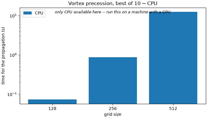
Time a vortex-pair propagation across grid sizes.

The timings are saved so they can be put next to the Julia implementation’s, so this measures propagation and nothing else – no sampling, no plotting. See vortex_precession_animation.py for the picture of what is propagating.

The step is fixed rather than left to the solver: a benchmark compares cost per unit of work, and letting each grid size choose its own step would change the work between the cells being compared.

CPU 128
Average time: 0.07 s (min: 0.07 s, max: 0.08 s)
CPU 256
/home/runner/work/NLSE/NLSE/NLSE/solvers/nlse.py:380: UserWarning: delta_z=2.18e-04 exceeds split-step accuracy limit (8.58e-05). Reducing to 7.72e-05.
  delta_z = self._capped_delta_z(delta_z, A, method)
Average time: 0.90 s (min: 0.87 s, max: 0.94 s)
CPU 512
/home/runner/work/NLSE/NLSE/NLSE/solvers/nlse.py:380: UserWarning: delta_z=2.18e-04 exceeds split-step accuracy limit (2.15e-05). Reducing to 1.93e-05.
  delta_z = self._capped_delta_z(delta_z, A, method)
Average time: 12.43 s (min: 12.37 s, max: 12.52 s)

import os
import time

import matplotlib.pyplot as plt
import numpy as np
from _output import output_path
from NLSE import NLSE
from NLSE.backends import list_available_backends


def vortex(x, y, xi=10e-6, ell=1):
    """Return the phase and density profile of a charge-``ell`` vortex."""
    r = np.hypot(x, y)
    theta = np.arctan2(x, y)
    return r / np.sqrt(r**2 + (xi / 0.83) ** 2) * np.exp(1j * ell * theta)


N = 256
n2 = -1.6e-10
waist = 750e-6
window = 3.5 * waist
power = 1.05
intensity = power / (np.pi * waist**2)
Isat = np.inf  # saturation intensity in W/m^2
L = 5e-2
alpha = 0
BACKENDS = list_available_backends()

# A solver at the reference size, only to get the healing length and the
# nonlinear length the step and the vortex separation are written against.
reference = NLSE(
    alpha, power, window, n2, None, L, NX=N, NY=N, Isat=Isat, backend=BACKENDS[0]
)
cs = np.sqrt(abs(n2) * intensity) / (1 + intensity / Isat)
delta_n = abs(n2) * intensity / (1 + intensity / Isat) ** 2
xi = 1 / (reference.k * cs)
z_nl = 1 / (reference.k * delta_n)
DELTA_Z = z_nl / 6

# A documentation build sets NLSE_DOCS_BUILD and gets the small sweep, so the
# gallery shows a real graph made by this script rather than a placeholder.
# Run it yourself and you get the full range.
sizes = (
    [128, 256, 512]
    if os.environ.get("NLSE_DOCS_BUILD")
    else [128, 256, 512, 1024, 2048, 4096, 8192]
)
navg = 10
# Every backend on the same grids, because a timing against nothing is not a
# benchmark: the comparison between them is what the figure is for.
ts = np.zeros((len(BACKENDS), len(sizes), navg))
for b, backend in enumerate(BACKENDS):
    for i, n in enumerate(sizes):
        print(f"{backend} {n}")
        simu = NLSE(
            alpha, power, window, n2, None, L, NX=n, NY=n, Isat=Isat, backend=backend
        )
        # A vortex pair, separated by four healing lengths.
        d = 4 * xi
        E_0 = np.exp(-(simu.XX**2 + simu.YY**2) / waist**2).astype(np.complex64)
        E_0 *= vortex(simu.XX + d / 2, simu.YY + d / 2, xi=xi, ell=1)
        E_0 *= vortex(simu.XX - d / 2, simu.YY - d / 2, xi=xi, ell=1)
        # Hand tuned potential for Thomas-Fermi
        simu.V = 4.31e-4 * np.exp(-2 * (simu.XX**2 + simu.YY**2) / waist**2).astype(
            np.float32
        )
        for rep in range(navg):
            t0 = time.perf_counter()
            simu.out_field(
                E_0,
                simu.L,
                verbose=False,
                plot=False,
                splitting="lie",
                delta_z=DELTA_Z,
            )
            ts[b, i, rep] = time.perf_counter() - t0
        timing_string = f"Average time: {np.mean(ts[b, i]):.2f} s "
        timing_string += (
            f"(min: {np.min(ts[b, i]):.2f} s, max: {np.max(ts[b, i]):.2f} s)"
        )
        print(timing_string)

for b, backend in enumerate(BACKENDS):
    np.save(output_path(f"python_vortex_precession_{backend}_times.npy"), ts[b])
    np.save(output_path(f"python_vortex_precession_{backend}_sizes.npy"), sizes)

# The timings are the point of the script, so draw them rather than leaving
# the reader to open a .npy. Best of the repeats, which is the figure least
# disturbed by whatever else the machine was doing.
best = ts.min(axis=2)
fig, ax = plt.subplots(figsize=(7, 4), constrained_layout=True)
width = 0.8 / len(BACKENDS)
offsets = np.arange(len(sizes))
for b, backend in enumerate(BACKENDS):
    ax.bar(offsets + b * width, best[b], width, label=backend)
ax.set_xticks(offsets + width * (len(BACKENDS) - 1) / 2)
ax.set_xticklabels([str(size) for size in sizes])
ax.set_yscale("log")
ax.set_xlabel("grid size")
ax.set_ylabel("time for the propagation (s)")
ax.set_title(f"Vortex precession, best of {navg} -- {', '.join(BACKENDS)}")
# A backend comparison is only a comparison if there is more than one backend.
# The documentation runner has no GPU and no OpenCL, so the figure published
# with these docs has a single bar; say so on it rather than let a reader take
# CPU-only for the whole story.
if len(BACKENDS) == 1:
    ax.text(
        0.5,
        0.94,
        f"only {BACKENDS[0]} available here -- run this on a machine with a GPU",
        transform=ax.transAxes,
        ha="center",
        fontsize=9,
        style="italic",
    )
ax.legend()
plt.show()