Physical validation

Most of a solver’s test suite can pass while the physics is wrong. Tests that compare the backends against each other pass when all of them are wrong in the same way. Tests that measure convergence order pass when the answer converges beautifully to the wrong number — order is a statement about how the error shrinks, not about what it shrinks towards. And a test that checks the propagator by writing the same formula a second time and comparing catches a typo in one of the two copies, never the formula itself.

So there is a separate suite, tests/physics/test_closed_forms.py, whose assertions come from outside the package: solutions of the same equation that were known before this code existed. Each one isolates a different term, and the last one isolates none of them.

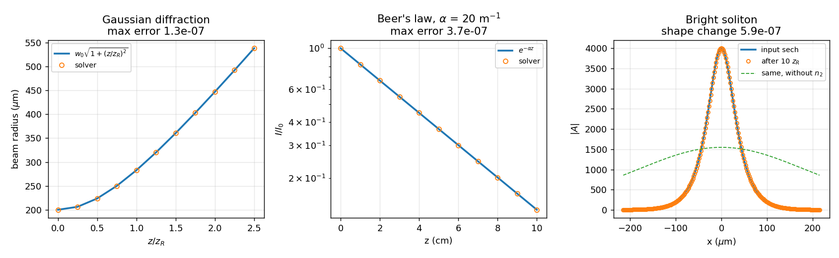
Curves are the analytic solutions, markers are what the solver returns. The residuals in the titles are what the figure cannot show.

The equation, and the conventions it fixes

\[ i\frac{\partial A}{\partial z} = -\frac{1}{2k}\nabla^2 A - k\,n_2\,\frac{I}{1 + I/I_{sat}}\,A, \qquad I = \frac{c\varepsilon_0}{2}|A|^2 \]

Two conventions follow from it that nothing else in the documentation stated, and that the tests now pin:

• \(n_2 > 0\) is self-focusing. A positive nonlinear index raises the index where the beam is brightest, which is what makes the bright soliton below exist at that sign and not the other.

• alpha attenuates the intensity, not the amplitude: \(I = I_0e^{-\alpha z}\). A factor of two here is invisible to every other kind of test.

What each check isolates

Check	Closed form	Isolates	Agreement
Gaussian diffraction	\(w(z) = w_0\sqrt{1 + (z/z_R)^2}\), \(z_R = kw_0^2/2\)	the propagator, its normalization, the \(k\) grid, the wavelength	exact
Gouy phase	\(\varphi(0,z) = -\arctan(z/z_R)\)	the sign and scale of the dispersion relation	5 decimals
Talbot revival	\(z_T = kd^2/\pi\)	the propagator at a finite transverse wavenumber	\(1.6\times10^{-6}\)
Beer’s law	\(I(z) = I_0e^{-\alpha z}\)	the loss term, and its convention	6 decimals
Saturated self-phase modulation	\(\varphi = k n_2 I z / (1 + I/I_{sat})\)	the interaction term and the saturation model	\(10^{-7}\)
The lossy identity	\(\varphi = \dfrac{k n_2}{\alpha}\left(I_0 - I_{end}\right)\)	loss and interaction together	\(4\times10^{-7}\)
Bright soliton	\(x_0^2 = 1/(k g A_0^2)\), \(g = kn_2c\varepsilon_0/2\)	nothing separately — only the balance	\(6\times10^{-7}\)

Why three checks on the propagator

A beam diffracts at roughly the right rate under a surprising range of mistakes, and a second moment is a blunt instrument. The Gouy phase is the sharp one: flipping the sign of the dispersion operator still produces a beam that spreads, and only the phase test notices. The Talbot distance covers what neither can — both Gaussian tests concentrate their power near \(K = 0\), where a wrong dispersion relation hides, while a grating puts all of it at one finite \(K\) and revives only at the distance that \(K^2/2k\) predicts.

The lossy identity

This one is worth stating in full, because it is the physics behind the solved real-space step rather than a property of the numerics. With \(y = |A|^2\) and \(s = 1/(1 + y/I_{sat})\),

\[ \frac{\mathrm{d}y}{\mathrm{d}z} = -\alpha s y, \qquad \frac{\mathrm{d}\varphi}{\mathrm{d}z} = k n_2 y s \qquad\Longrightarrow\qquad \frac{\mathrm{d}\varphi}{\mathrm{d}y} = -\frac{k n_2}{\alpha} \]

so the phase accumulated over any distance depends only on how much intensity was lost, whatever the saturation did in between — and the intensity that remains is fixed implicitly by \(\ln I + I/I_{sat}\) falling by \(\alpha z\). Both halves are asserted. Elsewhere the suite measures the order of that step; here it is measured against the answer.

The soliton, and its control

\(A_0\,\mathrm{sech}(x/x_0)\) propagates unchanged only when diffraction and self-focusing cancel exactly. Every other check above passes if the two terms are individually right; this is the one that fails if a sign or a factor sits between them. It is asserted alongside a control — the same profile 1.5x too wide, which is not a soliton and visibly spreads — because “the shape barely changed” means nothing without something that changed.

What breaking the physics does

The checks were verified by breaking the solver on purpose. Each mutation is a plausible slip in a constant that no other test in the suite reads against anything external:

Injected fault	Caught by
dispersion off by a factor of two	diffraction, Gouy, Talbot
dispersion sign flipped	Gouy only
alpha applied whole instead of halved	Beer, the lossy identity
saturation off by a factor of two	Beer, the lossy identity

What this does not cover

• Vortex dynamics. A vortex–antivortex pair should translate at \(v = \hbar/(md)\), which is the natural closed form for a periodic box since net circulation must vanish there. A first attempt reproduced it to 7% at one separation and not at two others; the initial state was not relaxed and the core positions came out quantized to the grid. Doing it properly needs imaginary-time relaxation and sub-pixel core fitting, and a test that passes at one separation is worse than none.

• The absorbing potential and the coupled solvers. Their real-space step is still frozen rather than solved, so it is first order in a lossy medium. That is a known limitation rather than an untested one — see the Open section of docs/optimization-log.md.

• Whether the grid resolves your problem. Every check here is self-consistent on its own grid. None of them says that the grid you chose is fine enough for the physics you are running.