Solvers Overview¶

All solvers share a common interface inherited from the base NLSE class. This page covers the solver hierarchy, features, and usage patterns.

Inheritance¶

All solver classes inherit from the main NLSE class to minimize code duplication:

inheritance

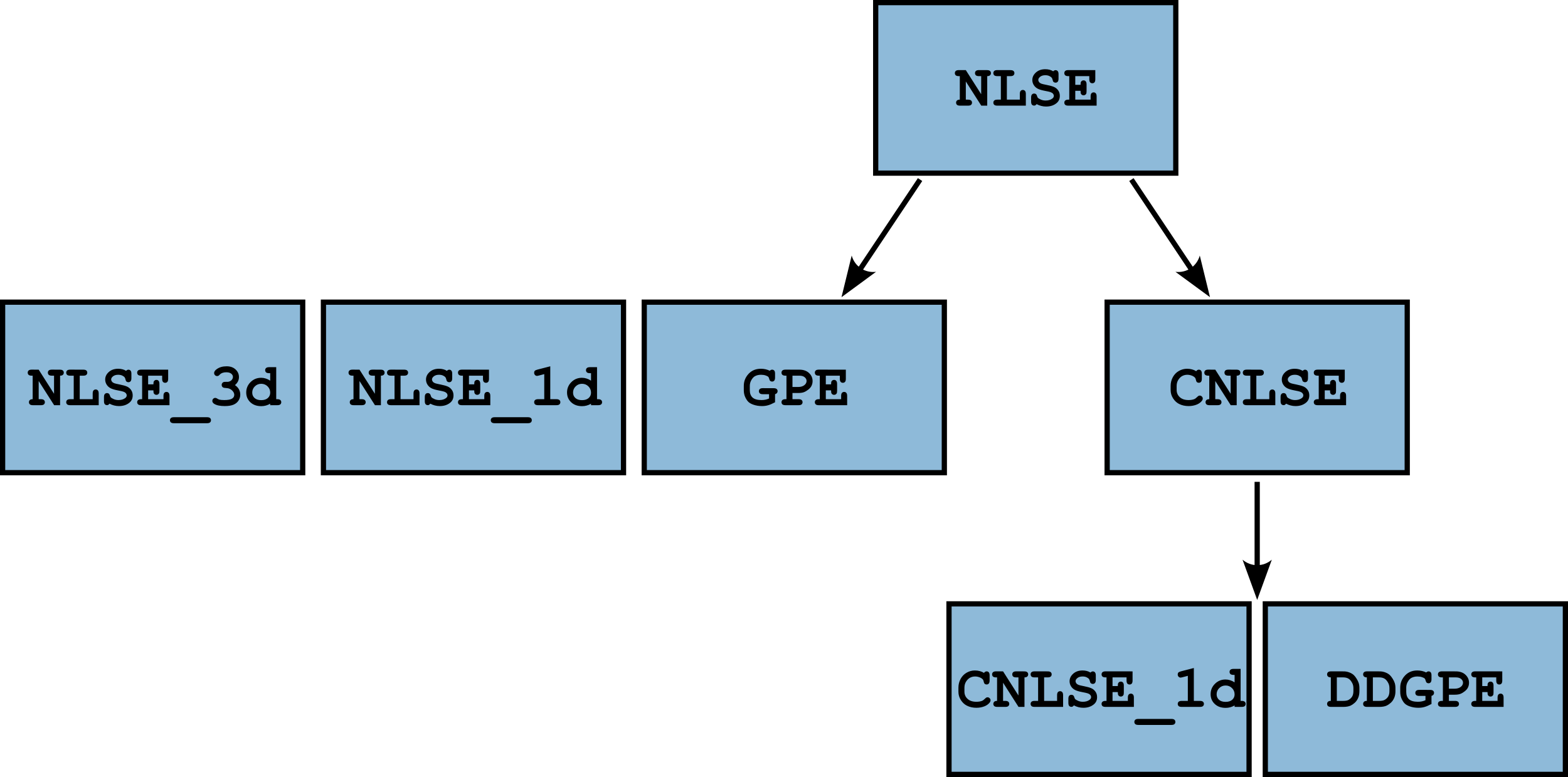
NLSE (2D base class)
├── NLSE_1d          - 1D specialization
├── NLSE_3d          - 3D+1 paraxial propagation
├── CNLSE            - Coupled NLSE (two-component)
│   ├── CNLSE_1d     - 1D coupled
│   └── DDGPE        - Driven-dissipative GPE
└── GPE              - Gross-Pitaevskii equation

Solver Comparison¶

Solver	Dimensions	Components	Unit system	Non-locality	GVD
`NLSE`	2D	1	Optics (SI)	Yes	No
`NLSE_1d`	1D	1	Optics (SI)	Yes	No
`NLSE_3d`	3D	1	Optics (SI)	No	Yes
`CNLSE`	2D	2	Optics (SI)	No	No
`CNLSE_1d`	1D	2	Optics (SI)	No	No
`GPE`	2D	1	Atomic (SI)	Yes	No
`DDGPE`	2D	2	Polariton	No	No

The equation each solver integrates¶

NLSE itself is the 2D paraxial equation set out in Physics Background; the rest specialise or extend it.

The `NLSE_1d` class¶

NLSE_1d is a 1D specialization of NLSE for performance. It supports all of the features of the main NLSE class.

The propagation equation is:

\[ i\partial_{z}E = -\frac{1}{2k_0}\partial^2_x E + -\frac{k_0}{2}\delta n(r) E - n_2 \frac{k_0}{2n}c\epsilon_0|E|^2E \]

The `NLSE_3d` class¶

NLSE_3d solves the full paraxial propagation equation.

WARNING: Since this solves a 3D+1 equation, this is computationally very intensive ! The space complexity scales as \(N^3\) if \(N\) is the field array size.

The propagation equation is:

\[ i\partial_{z}E = -\frac{1}{2k_0}\nabla_{\perp}^2 E + \frac{D_0}{2}\partial^2_t E -\frac{k_0}{2}\delta n(r) E - n_2 \frac{k_0}{2n}c\epsilon_0|E|^2E \]

The `CNLSE` class¶

The CNLSE class is a coupled non-linear Schrödinger equation allowing to solve the following equation:

\[\begin{split} \begin{split} i\frac{\partial\psi_f}{\partial z} &= -\frac{1}{2k_f}\nabla^2\psi_f -\frac{1}{2}n_2^f k_f c\epsilon_0|\psi_f|^2\psi_f + k_f n_2^{fd}c\epsilon_0|\psi_d|^2\psi_f-\frac{i\alpha_f}{2}\psi_f + \frac{\Omega}{2} \psi_d \\ i\frac{\partial\psi_d}{\partial z} &= -\frac{1}{2k_d}\nabla^2\psi_d -\frac{1}{2}n_2^d k_d c\epsilon_0|\psi_d|^2\psi_d + k_d n_2^{fd}c\epsilon_0|\psi_f|^2\psi_d-\frac{i\alpha_d}{2}\psi_d + \frac{\Omega}{2} \psi_f \end{split} \end{split}\]

This allows to describe the back reaction of the fluid onto the defect as well as two components scenarii. In order to “turn on” different terms, it suffices to set the parameters value to something other than None. When None, the solver does not apply the corresponding evolution term for optimal performance.

The `CNLSE_1d` class¶

Similarly to NLSE_1d, the CNLSE_1d is a 1D specialization of CNLSE class.

The propagation equation is:

\[\begin{split} \begin{split} i\frac{\partial\psi_f}{\partial z} &= -\frac{1}{2k_f}\partial^2_x\psi_f -\frac{1}{2}n_2^f k_f c\epsilon_0|\psi_f|^2\psi_f + k_f n_2^{fd}c\epsilon_0|\psi_d|^2\psi_f-\frac{i\alpha_f}{2}\psi_f + \frac{\Omega}{2} \psi_d \\ i\frac{\partial\psi_d}{\partial z} &= -\frac{1}{2k_d}\partial^2_x\psi_d -\frac{1}{2}n_2^d k_d c\epsilon_0|\psi_d|^2\psi_d + k_d n_2^{fd}c\epsilon_0|\psi_f|^2\psi_d-\frac{i\alpha_d}{2}\psi_d + \frac{\Omega}{2} \psi_f \end{split} \end{split}\]

The `GPE` class¶

The GPE class allows to solve the 2D Gross-Pitaevskii equation describing the temporal evolution of a Bosonic field:

\[ i\partial_{t}\psi = -\frac{1}{2}\nabla^2\psi+V\psi+g|\psi|^2\psi. \]

It follows exactly the same conventions as the other classes a part from the fact that since it describes atoms, the units are the “atomic” units (masses in kg, times in s).

The `DDGPE` class¶

The DDGPE class allows to solve the temporal evolution of two coupled fields in a driven-dissipative context.

It was designed to study problems like the evolution of exciton polaritons in microcavities.

The equation solved in this context is the following:

\[\begin{split} \begin{split} i\hbar \partial_t\psi_X(\textbf{r}, t)&= (\frac{\hbar^2}{2m_X}\nabla^2 + V_X(\textbf{r}) + \hbar g_X|\psi_X(\textbf{r}, t)|^2 - i\hbar\frac{\Gamma_X}{2})\psi_X(\textbf{r}, t)+ \hbar\Omega_R\psi_C(\textbf{r}, t) \\ i\hbar \partial_t \psi_C(\textbf{r}, t)&= (\frac{\hbar^2}{2m_C}\nabla^2 + V_C(\textbf{r}) - i\hbar\frac{\Gamma_C}{2})\psi_C(\textbf{r}, t) + \hbar\Omega_R\psi_X(\textbf{r}, t) + \hbar F_p(\textbf{r},t) \end{split} \end{split}\]

where

\(\psi_X\) is the exciton field
\(\psi_C\) is the cavity field
\(V_X\) is the exciton potential
\(V_C\) is the cavity potential
\(g_X\) is the exciton interaction energy
\(\Gamma_X\) is the exciton losses coefficient
\(\Gamma_C\) is the cavity losses coefficient
\(\Omega_R\) is the Rabi coupling between excitons and photons
\(F_p\) is the pumping field impinging on the cavity

Common Interface¶

All solvers are imported from the top-level package:

from NLSE import NLSE, NLSE_1d, NLSE_3d, CNLSE, CNLSE_1d, GPE, DDGPE

Creating a Solver¶

Each solver takes physical parameters at initialization:

simu = NLSE(
    alpha=20,           # linear losses (m^-1)
    power=1.05,         # optical power (W)
    window=8e-3,        # computational window (m), can be (wx, wy) tuple
    n2=-1.6e-9,         # nonlinear index (m^2/W)
    V=None,             # potential array or None
    L=10e-3,            # propagation distance (m)
    NX=1024,            # grid points in x
    NY=1024,            # grid points in y
    Isat=np.inf,        # saturation intensity (W/m^2)
    nl_length=0,        # non-local length (m), 0 = local
    wvl=780e-9,         # wavelength (m)
    backend="CPU",      # backend name
)

Propagation¶

The main entry point is out_field():

E_out = simu.out_field(
    E_in,                # input field (normalized 0-1)
    z,                   # propagation distance
    splitting="lie",  # "lie" O(dz), "strang" O(dz^2), "yoshida" O(dz^4)
    method="split_step", # "split_step" or "RK4"
    callback=None,       # callback function(s)
    callback_args=(),    # additional callback arguments
    plot=False,          # plot results
    verbose=True,        # print progress
    normalize=True,      # normalize to total power
)

The returned field E_out is always a NumPy array on the CPU, in physical units (V/m for optical solvers).

Coordinate Grids¶

After initialization, the solver provides coordinate arrays:

# 2D solvers (NLSE, CNLSE, GPE, DDGPE)
simu.X       # 1D x-coordinate array
simu.Y       # 1D y-coordinate array
simu.XX      # 2D meshgrid (x)
simu.YY      # 2D meshgrid (y)
simu.delta_X # grid spacing in x
simu.delta_Y # grid spacing in y

# 1D solvers (NLSE_1d, CNLSE_1d)
simu.X       # 1D coordinate array
simu.delta_X # grid spacing

# Fourier space
simu.Kx      # x spatial frequencies
simu.Ky      # y spatial frequencies
simu.Kxx     # 2D meshgrid of frequencies (x)
simu.Kyy     # 2D meshgrid of frequencies (y)

Setting the Potential¶

The potential can be set at initialization or later:

# At initialization
simu = NLSE(..., V=my_potential)

# After initialization
simu.V = my_potential

For 2D solvers, the potential should have shape (NY, NX). Set to None for free propagation.

Non-locality¶

nl_length models a diffusive non-locality, as a Bessel kernel convolved with the intensity. The kernel spans nl_length // delta_X grid cells, so the grid has to resolve the length you ask for: below one cell the kernel is a single point, which is the identity. The solver warns and propagates locally in that case rather than charging you for a convolution that does nothing.

Only CPU and CUPY have the convolution. Asking for a non-locality on OpenCL or MLX moves the solver to the fastest backend that has one, with a warning saying which and why — the backend is how a run goes, the non-locality is what it computes, and the physics is not the part to give up. See Backends.

Complex potentials¶

V may be complex. Its real part shifts the phase, as a refractive index change does; its imaginary part is gain or loss, entering the real part of the exponent rather than the phase. That is how an absorbing boundary is built:

import numpy as np
from NLSE import NLSE

waist = 2.23e-3
simu = NLSE(alpha=0, power=1.05, window=4 * waist, n2=-1.6e-9, V=None,
            L=10e-3, NX=256, NY=256, Isat=10e4)

# A ring of loss around the beam, to stop light wrapping around the window
r = np.hypot(simu.XX, simu.YY)
absorber = 1j * 2e2 * np.exp(-((r - 2e-3) ** 2) / (3e-4) ** 2)
simu.V = absorber.astype(np.complex64)

E_in = np.exp(-r**2 / waist**2).astype(np.complex64)
E_out = simu.out_field(E_in, 2e-3)

Positive imaginary part removes power, negative adds it. The potential is transferred at the field’s precision, so a complex64 field carries a complex64 potential and a complex128 one carries complex128.

Step Size¶

delta_z is an argument to out_field. Left out, the solver derives one from the field’s energy; passed, it is used as given:

E = simu.out_field(E_in, z, delta_z=1e-5)  # manual step size in meters

Either way the step is capped to the method’s region of convergence before propagation, with a warning if that binds (see Numerical Methods).

Coupled Solvers (CNLSE, CNLSE_1d, DDGPE)¶

Coupled solvers propagate two field components simultaneously. The input field has an extra leading dimension:

import numpy as np
from NLSE import CNLSE

waist, L = 2.23e-3, 10e-3
simu = CNLSE(
    alpha=20, power=1.05, window=8e-3,
    n2=-1.6e-9, V=None, L=10e-3,
    NX=512, NY=512,
    n12=-0.5e-9,   # cross-interaction coefficient
    omega=1e3,     # Rabi coupling
)

# Input: shape (2, NY, NX)
E_in = np.zeros((2, 512, 512), dtype=np.complex64)
E_in[0] = np.exp(-(simu.XX**2 + simu.YY**2) / waist**2)  # component 1
E_in[1] = 0  # component 2 starts empty

E_out = simu.out_field(E_in, L, splitting="lie")
# E_out.shape == (2, 512, 512)

Setting coupling parameters to None disables the corresponding term for better performance.

Broadcasting (Parallel Simulations)¶

You can run multiple simulations in parallel using NumPy broadcasting. This works on every backend. CUPY and MLX hand the batched parameters to their kernels and broadcast there; CPU and OpenCL take one simulation’s values per launch and loop over the batch, so their gain over separate runs is in the FFTs rather than in the kernels.

# Propagate 10 different initial states
E_in = np.random.randn(10, NY, NX) + 1j * np.random.randn(10, NY, NX)
E_out = simu.out_field(E_in, L)
# E_out.shape == (10, NY, NX)

# Scan over n2 values, same initial state for each
field = np.exp(-(simu.XX**2 + simu.YY**2) / waist**2).astype(np.complex64)
simu.n2 = np.linspace(-2e-9, -1e-9, 5).reshape(5, 1, 1)
E_in = np.broadcast_to(field, (5, NY, NX)).copy()
E_out = simu.out_field(E_in, L)

# Grid search over two parameters
N_n2, N_alpha = 5, 3
simu.n2 = np.linspace(-2e-9, -1e-9, N_n2).reshape(N_n2, 1, 1, 1)
simu.alpha = np.linspace(0, 20, N_alpha).reshape(1, N_alpha, 1, 1)
E_in = np.broadcast_to(field, (N_n2, N_alpha, NY, NX)).copy()
E_out = simu.out_field(E_in, L)

Array shapes must follow NumPy broadcasting rules.

Note

The batch axes come first and the grid axes last, so a scan over two parameters on a 2D grid is a four-dimensional array. Memory is the limit: every simulation in the batch holds its own field.

Plotting¶

All solvers have a plot_field method for visualizing fields:

simu.plot_field(E_out)

Solvers Overview¶

Inheritance¶

Solver Comparison¶

The equation each solver integrates¶

The NLSE_1d class¶

The NLSE_3d class¶

The CNLSE class¶

The CNLSE_1d class¶

The GPE class¶

The DDGPE class¶

Common Interface¶

Creating a Solver¶

Propagation¶

Coordinate Grids¶

Setting the Potential¶

Non-locality¶

Complex potentials¶

Step Size¶

Coupled Solvers (CNLSE, CNLSE_1d, DDGPE)¶

Broadcasting (Parallel Simulations)¶

Plotting¶

The `NLSE_1d` class¶

The `NLSE_3d` class¶

The `CNLSE` class¶

The `CNLSE_1d` class¶

The `GPE` class¶

The `DDGPE` class¶