Spin and density modes¶

The two Bogoliubov branches of a binary fluid of light, after Piekarski et al., Phys. Rev. Lett. 134, 223403 (2025).

Two circular polarisations propagating through the same vapour are two fluids that see each other. Perturb them together and the medium resists with the sum of the interactions; perturb them against each other and it resists with the difference. So a binary fluid has two speeds of sound rather than one, and two dispersion branches to go with them:

\[\Omega_{d,s}(k) = \sqrt{\left(\frac{k^2}{2k_0}\right)^2 + k^2 c_{d,s}^2}\]

This page measures both, the way the experiment does – imprint a small sinusoidal modulation of wavenumber $k$, watch the fringe contrast oscillate along the cell, read the frequency off it – and then does the thing that makes the paper: turns the intensity up until the two branches cross.

Why they cross is worth stating carefully, because it is not obvious. The medium saturates, so the index depression is $\Delta n = n_2 I/(1+I/I_{sat})$, and the restoring force for each mode is the derivative of that along its own direction in the space of the two densities. The density mode moves the total intensity, so the saturation denominator gets differentiated too and comes back squared. The spin mode moves intensity from one component to the other at fixed total, so the denominator is a constant for it and appears only once:

\[c_d^2 = \frac{(|n_2|+|n_{12}|)\,I_0/2}{(1+I_0/I_{sat})^2}, \qquad c_s^2 = \frac{(|n_2|-|n_{12}|)\,I_0/2}{1+I_0/I_{sat}}\]

At low intensity the first is the larger, as the two-body picture says it must be: $g+g_{12}$ beats $g-g_{12}$. But it also falls off faster, so somewhere the ordering reverses – at

\[\frac{I_0}{I_{sat}} = \frac{2|n_{12}|}{|n_2|-|n_{12}|}\]

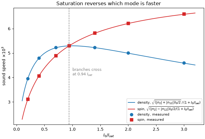
which for the measured ratio $|n_{12}|/|n_2| = 0.32$ is $I_0 \simeq 0.94\,I_{sat}$, comfortably inside the range a vapour cell reaches. Past it the spin mode is the faster one, which no two-body interaction can produce.

The perturbation only varies along one transverse direction, so this runs on CNLSE_1d and the whole page costs a few seconds.

import matplotlib.pyplot as plt
import numpy as np
from NLSE import CNLSE_1d
from scipy.constants import c as c_light, epsilon_0

The medium, measured. n2 is the circular-polarisation value from the paper and n12/n2 its fitted ratio; the saturation intensity is what the crossing is measured against, so it is the one number the result is most sensitive to.

# Only two ratios decide where the branches cross -- |n12|/|n2| and
# I0/Isat -- so the measured ones are kept and |n2| is not. The paper's
# -3.9e-11 m^2/W puts one Bogoliubov period at 0.8 m, which is why the
# experiment reads contrast extrema across a 5 cm cell rather than counting
# oscillations; a stronger medium puts several periods in a 30 cm cell and
# lets the frequency be read directly, at no cost to the physics on show.
RATIO = 0.32  # |n12|/|n2|, fitted in the paper
I_SAT = 17e4  # W/m^2 (17 W/cm^2), measured
N2 = -1e-9  # m^2/W; the paper's is -3.9e-11, see above
N12 = RATIO * N2
WVL = 795e-9  # rubidium D1
K0 = 2 * np.pi / WVL
N_PTS = 256


def speeds(i0):
    """Return the closed-form density and spin sound speeds.

    Parameters
    ----------
    i0 : float or ndarray
        Total intensity in W/m^2.

    Returns
    -------
    tuple
        ``(c_d, c_s)``, dimensionless (angles, as every speed here is).
    """
    saturation = 1 + i0 / I_SAT
    c_d = np.sqrt((abs(N2) + abs(N12)) * (i0 / 2)) / saturation
    c_s = np.sqrt((abs(N2) - abs(N12)) * (i0 / 2) / saturation)
    return c_d, c_s


CROSSING = 2 * abs(N12) / (abs(N2) - abs(N12))
print(f"branches cross at I0/Isat = {CROSSING:.2f}")


def dispersion(k, c):
    """Bogoliubov frequency at wavenumber ``k`` for sound speed ``c``.

    Parameters
    ----------
    k : float or ndarray
        Transverse wavenumber in rad/m.
    c : float or ndarray
        Sound speed.

    Returns
    -------
    float or ndarray
        Spatial frequency along z, in rad/m.
    """
    return np.sqrt((k**2 / (2 * K0)) ** 2 + k**2 * c**2)


def measure(i0, mode, k_xi=1.0, periods=12):
    r"""Imprint one Bogoliubov mode and read its frequency off the propagation.

    The perturbation is applied in phase for the density mode and in
    antiphase for the spin mode, which is the same selection rule the
    experiment implements by choosing the polarisation angle of its Bragg
    beams. Its Fourier amplitude then oscillates along z at exactly
    :math:`\Omega`, and fitting that oscillation is the measurement.

    Parameters
    ----------
    i0 : float
        Total intensity in W/m^2.
    mode : str
        ``"density"`` or ``"spin"``.
    k_xi : float
        Perturbation wavenumber in units of 1/xi. At 1 the two terms of the
        dispersion are comparable, which is where inverting it for the sound
        speed is best conditioned.
    periods : int
        How many oscillations to propagate for.

    Returns
    -------
    tuple of float
        The measured frequency and the sound speed inferred from it.
    """
    # The scales, from the mode being measured: each branch has its own.
    c_d, c_s = speeds(i0)
    c_expected = c_d if mode == "density" else c_s
    xi = 1 / (K0 * c_expected)
    k_p = k_xi / xi
    omega_expected = dispersion(k_p, c_expected)
    length = periods * 2 * np.pi / omega_expected

    # A whole number of periods of the perturbation has to fit the window, or
    # it does not close on the periodic grid and the seam radiates.
    modes = 8
    window = modes * 2 * np.pi / k_p
    k_p = 2 * np.pi * modes / window

    # The same Nyquist stability bound as the soliton example: the linear
    # phase per step at the grid's highest wavenumber has to stay near a
    # radian, or the background destabilises and the "measurement" is of the
    # numerics rather than the fluid.
    dx = window / N_PTS
    delta_z = 1.0 * 2 * K0 / (np.pi / dx) ** 2

    simu = CNLSE_1d(
        0, 1.0, window, N2, N12, None, length, NX=N_PTS, Isat=I_SAT, wvl=WVL
    )
    simu.n22 = N2  # one medium: each component sees itself as it sees itself
    simu.I_sat2 = I_SAT
    simu.alpha2 = 0.0

    # The amplitude is set from the intensity wanted rather than left to the
    # solver's power normalisation, and ``normalize=False`` below keeps it.
    # What ``power`` means is unambiguous in 2D -- the integral of the
    # intensity over the window -- but this is the 1D solver, where following
    # that convention would put the background intensity out by a factor of
    # the grid pitch. Saturation makes the absolute intensity physical here,
    # not just a scale, so it is worth being explicit about.
    amplitude = np.sqrt(2 * (i0 / 2) / (c_light * epsilon_0))
    epsilon = 0.02
    ripple = epsilon * np.cos(k_p * simu.X)
    sign = +1 if mode == "density" else -1
    E = (
        amplitude
        * np.array(
            [np.ones(N_PTS) * (1 + ripple), np.ones(N_PTS) * (1 + sign * ripple)]
        )
    ).astype(np.complex64)

    signal, zs = [], []

    def watch(sim, A, z, i):
        """Record the perturbation's Fourier amplitude at k_p."""
        if i % 20:
            return
        host = np.asarray(sim._backend.to_numpy(A))
        i1, i2 = np.abs(host[0]) ** 2, np.abs(host[1]) ** 2
        combination = i1 + sign * i2
        combination = combination - combination.mean()
        spectrum = np.fft.rfft(combination)
        signal.append(spectrum[modes].real)
        zs.append(z)

    simu.out_field(
        E,
        length,
        delta_z=delta_z,
        verbose=False,
        plot=False,
        callback=watch,
        normalize=False,
    )

    # The frequency, from the peak of the signal's own spectrum, refined by a
    # parabolic fit so it is not quantised to the bin spacing.
    signal = np.asarray(signal, dtype=float)
    zs = np.asarray(zs)
    signal = signal - signal.mean()
    power = np.abs(np.fft.rfft(signal * np.hanning(signal.size)))
    peak = int(np.argmax(power[1:]) + 1)
    if 0 < peak < power.size - 1:
        left, mid, right = power[peak - 1 : peak + 2]
        peak = peak + 0.5 * (left - right) / (left - 2 * mid + right)
    omega = 2 * np.pi * peak / (zs[-1] - zs[0])

    # Invert the dispersion for the sound speed, which is what is compared.
    free = k_p**2 / (2 * K0)
    c_measured = np.sqrt(max(omega**2 - free**2, 0.0)) / k_p
    return omega, c_measured

branches cross at I0/Isat = 0.94

One measurement, to show what is being read. At $I_0 = I_{sat}$ the two branches are nearly on top of each other – the crossing is at $0.94\,I_{sat}$ – so this is the least favourable place to try to tell them apart, and they still come out right.

for mode in ("density", "spin"):
    omega, c = measure(I_SAT, mode)
    c_d, c_s = speeds(I_SAT)
    expected = c_d if mode == "density" else c_s
    print(
        f"{mode:>8}: c = {c:.3e} measured, {expected:.3e} predicted "
        f"({100 * (c / expected - 1):+.1f}%)"
    )

 density: c = 5.309e-03 measured, 5.296e-03 predicted (+0.2%)
/home/runner/work/NLSE/NLSE/NLSE/solvers/nlse.py:380: UserWarning: delta_z=3.42e-05 exceeds split-step accuracy limit (3.42e-05). Reducing to 3.08e-05.
  delta_z = self._capped_delta_z(delta_z, A, method)
    spin: c = 5.387e-03 measured, 5.376e-03 predicted (+0.2%)

The scan. Walking the intensity across the crossing, the density branch falls behind the spin branch and the ordering that the two-body picture insists on is broken. The lines are the closed forms above, the points the propagation.

intensities = I_SAT * np.array([0.2, 0.4, 0.7, 0.94, 1.4, 2.0, 3.0])
measured = {
    mode: np.array([measure(i0, mode)[1] for i0 in intensities])
    for mode in ("density", "spin")
}

grid = np.linspace(0.1, 3.2, 200) * I_SAT
c_d_grid, c_s_grid = speeds(grid)

print("\n I0/Isat   c_d meas   c_d calc   c_s meas   c_s calc")
for i0, cd, cs in zip(intensities, measured["density"], measured["spin"]):
    cd0, cs0 = speeds(i0)
    print(f"{i0 / I_SAT:8.2f} {cd:10.3e} {cd0:10.3e} {cs:10.3e} {cs0:10.3e}")

fig, ax = plt.subplots(figsize=(6.8, 4.6), layout="constrained")
ax.plot(
    grid / I_SAT,
    c_d_grid * 1e3,
    "-",
    color="tab:blue",
    label=r"density, $\sqrt{(|n_2|+|n_{12}|)I_0/2}\,/\,(1+I_0/I_{sat})$",
)
ax.plot(
    grid / I_SAT,
    c_s_grid * 1e3,
    "-",
    color="tab:red",
    label=r"spin, $\sqrt{(|n_2|-|n_{12}|)I_0/2/(1+I_0/I_{sat})}$",
)
ax.plot(
    intensities / I_SAT,
    measured["density"] * 1e3,
    "o",
    color="tab:blue",
    ms=7,
    label="density, measured",
)
ax.plot(
    intensities / I_SAT,
    measured["spin"] * 1e3,
    "s",
    color="tab:red",
    ms=7,
    label="spin, measured",
)
ax.axvline(CROSSING, color="gray", ls="--", lw=1.1)
ax.annotate(
    f"branches cross\nat {CROSSING:.2f} $I_{{sat}}$",
    xy=(CROSSING, 0.45),
    xycoords=("data", "axes fraction"),
    xytext=(8, 0),
    textcoords="offset points",
    va="center",
    fontsize=9,
    color="gray",
)
ax.set_xlabel(r"$I_0 / I_{sat}$")
ax.set_ylabel(r"sound speed $\times 10^{3}$")
ax.set_title("Saturation reverses which mode is faster")
ax.legend(fontsize=8)
plt.show()

Saturation reverses which mode is faster

/home/runner/work/NLSE/NLSE/NLSE/solvers/nlse.py:380: UserWarning: delta_z=3.96e-05 exceeds split-step accuracy limit (3.96e-05). Reducing to 3.57e-05.
  delta_z = self._capped_delta_z(delta_z, A, method)
/home/runner/work/NLSE/NLSE/NLSE/solvers/nlse.py:380: UserWarning: delta_z=3.53e-05 exceeds split-step accuracy limit (3.53e-05). Reducing to 3.18e-05.
  delta_z = self._capped_delta_z(delta_z, A, method)

 I0/Isat   c_d meas   c_d calc   c_s meas   c_s calc
    0.20  3.957e-03  3.948e-03  3.111e-03  3.104e-03
    0.40  4.797e-03  4.785e-03  4.074e-03  4.064e-03
    0.70  5.226e-03  5.213e-03  4.890e-03  4.879e-03
    0.94  5.306e-03  5.294e-03  5.303e-03  5.292e-03
    1.40  5.235e-03  5.222e-03  5.820e-03  5.807e-03
    2.00  5.004e-03  4.993e-03  6.221e-03  6.208e-03
    3.00  4.598e-03  4.587e-03  6.597e-03  6.584e-03

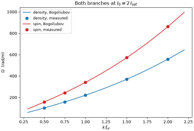
And the dispersion itself, at an intensity past the crossing, which is the quantity the Bragg spectroscopy actually returns. Both branches are measured at several wavenumbers and compared with the closed form; the free-particle term $k^2/2k_0$ is common to both, so everything that distinguishes them lives at small $k$.

i0 = 2.0 * I_SAT
k_values = np.array([0.5, 0.75, 1.0, 1.5, 2.0])
fig, ax = plt.subplots(figsize=(6.8, 4.6), layout="constrained")
for mode, colour in (("density", "tab:blue"), ("spin", "tab:red")):
    c_theory = speeds(i0)[0 if mode == "density" else 1]
    xi = 1 / (K0 * c_theory)
    ks, omegas = [], []
    for k_xi in k_values:
        omega, _ = measure(i0, mode, k_xi=k_xi, periods=10)
        ks.append(k_xi / xi), omegas.append(omega)
    smooth = np.linspace(0.3, 2.2, 100) / xi
    ax.plot(
        np.array(smooth) * xi,
        dispersion(smooth, c_theory),
        "-",
        color=colour,
        label=f"{mode}, Bogoliubov",
    )
    ax.plot(
        np.array(ks) * xi, omegas, "o", color=colour, ms=7, label=f"{mode}, measured"
    )
ax.set_xlabel(r"$k\,\xi_d$")
ax.set_ylabel(r"$\Omega$  (rad/m)")
ax.set_title(rf"Both branches at $I_0 = {i0 / I_SAT:.0f}\,I_{{sat}}$")
ax.legend(fontsize=9)
plt.show()

$Both branches at $I_0 = 2\,I_{sat}$$

/home/runner/work/NLSE/NLSE/NLSE/solvers/nlse.py:380: UserWarning: delta_z=1.59e-04 exceeds split-step accuracy limit (1.59e-04). Reducing to 1.43e-04.
  delta_z = self._capped_delta_z(delta_z, A, method)
/home/runner/work/NLSE/NLSE/NLSE/solvers/nlse.py:380: UserWarning: delta_z=7.05e-05 exceeds split-step accuracy limit (7.05e-05). Reducing to 6.34e-05.
  delta_z = self._capped_delta_z(delta_z, A, method)
/home/runner/work/NLSE/NLSE/NLSE/solvers/nlse.py:380: UserWarning: delta_z=1.76e-05 exceeds split-step accuracy limit (1.76e-05). Reducing to 1.59e-05.
  delta_z = self._capped_delta_z(delta_z, A, method)
/home/runner/work/NLSE/NLSE/NLSE/solvers/nlse.py:380: UserWarning: delta_z=9.91e-06 exceeds split-step accuracy limit (9.91e-06). Reducing to 8.92e-06.
  delta_z = self._capped_delta_z(delta_z, A, method)

Total running time of the script: (0 minutes 17.410 seconds)

Gallery generated by Sphinx-Gallery