Rayleigh-Taylor instability

A heavy fluid resting on a light one is unstable, and the fluid of light is no exception: the interface corrugates, the corrugations sharpen into fingers, and the fingers roll up into mushrooms. This page grows seven of them.

The two fluids are the two components of a coupled NLSE, made immiscible by a cross-coupling above the miscibility threshold, \(|n_{12}| > \sqrt{|n_2 n_{22}|}\). Their density contrast is bought with unequal self-interactions rather than unequal powers: at equal pressure \(|n_2| I_1 = |n_{22}| I_2\), so a component that repels itself three times less strongly sits three times denser, giving an Atwood number \(A = (n_1 - n_2)/(n_1 + n_2) = 0.5\) uniformly across the cloud.

The gravity is the trap itself. A confined cloud already carries \(\nabla p = -n\nabla U\) everywhere, so at radius \(r_0\) a fluid element feels an inward acceleration \(C r_0\). Put the dense component in an outer shell and the light one in the core and the arrangement is top-heavy: the shell falls inward through the core, which rises outward in fingers. Two things follow that a flat interface would not give. The circumference sets how many fingers fit – \(2\pi r_0/\lambda_\mathrm{fast}\) – and it selects them cleanly, because every azimuthal mode sees the same acceleration.

Note

A uniform index ramp added to a harmonic trap is not a way to do this. \(-Cr^2 - Gx\) is a displaced parabola, and at its minimum – where the interface would sit – the net force is zero. The ramp moves the cloud and drives nothing.

Warning

The trap is what makes the growth observable, and it is not accessible in the experiment for now. A freely propagating beam expands at the speed of sound, so its core survives only \(L < X/c_s\), while keeping the density positive caps the drive at \(g < \mu/X\). Together these give \(\gamma L_\mathrm{max}\sim(X/\xi)^{1/4}\), under two e-foldings and almost independent of how large the beam is made. This example is a numerical demonstration of the instability, not a simulation of a measurement.

What is checked here is the linear theory, in both of the numbers it offers. The azimuthal mode that grows comes out at 7 against a predicted 8.2, and the interface roughens exponentially at 11 m⁻¹ against a predicted 16. Both predictions carry the surface tension of the immiscible interface – without it every short wavelength would grow fastest and the ring would simply shatter rather than choose a mode – and its coefficient is only known to order unity, which is about the size of the discrepancy.

import matplotlib.pyplot as plt
import numpy as np
from matplotlib.animation import FuncAnimation
from NLSE import CNLSE
from scipy.constants import c, epsilon_0

# --- the two fluids ---------------------------------------------------------
WVL = 780e-9
K0 = 2 * np.pi / WVL
N2, N22 = -1e-9, -3e-9
# Just above the miscibility threshold. Far above it the interface is stiff and
# surface tension stabilises every mode the cloud can hold.
KAPPA = 1.10
N12 = -KAPPA * np.sqrt(abs(N2 * N22))
I_PEAK = 1.5e5

# --- the trap, and the ring inside it ---------------------------------------
R_TF = 1.8e-3
# Thomas-Fermi: both components share p = C (r_TF^2 - r^2) and differ only by
# their own g, so pressure balance and a uniform Atwood number come out of the
# construction rather than being tuned.
C_TRAP = 2 * abs(N2) * I_PEAK / R_TF**2
R0 = 0.6 * R_TF
ATWOOD = 0.5

WINDOW, N_PTS = 5e-3, 1152
TAU_END, N_FRAMES = 300, 40

# --- scales -----------------------------------------------------------------
MU = abs(N2) * I_PEAK
XI = 1 / (K0 * np.sqrt(MU))
Z_NL = K0 * XI**2
LENGTH = TAU_END * Z_NL
# At the interface the cloud has thinned, and it is the local healing length
# that sets both the interface width and the stabilising surface tension.
I_LOCAL = I_PEAK * (1 - (R0 / R_TF) ** 2)
MU_LOCAL = abs(N2) * I_LOCAL
XI_LOCAL = 1 / (K0 * np.sqrt(MU_LOCAL))
WIDTH = XI_LOCAL / np.sqrt(KAPPA - 1)

# --- the linear prediction --------------------------------------------------
# gamma^2 = A a k - sigma k^3 / rho: gravity grows every mode, surface tension
# kills the short ones. sigma ~ mu xi sqrt(kappa - 1) near threshold, which
# puts the cut-off at k_max and the fastest growth at k_max / sqrt(3).
ACC = C_TRAP * R0
K_MAX = np.sqrt(ATWOOD * ACC / (0.75 * MU_LOCAL * XI_LOCAL * np.sqrt(KAPPA - 1)))
K_FAST = K_MAX / np.sqrt(3)
M_FAST = 2 * np.pi * R0 * K_FAST / (2 * np.pi)
GAMMA = np.sqrt(ATWOOD * ACC * K_FAST * 2 / 3)

print(f"xi at the interface   {XI_LOCAL * 1e6:.1f} um")
print(f"acceleration C r0     {ACC:.3f} /m")
print(f"fastest wavelength    {2 * np.pi / K_FAST * 1e6:.0f} um")
print(f"predicted fingers     {M_FAST:.1f}")
print(f"predicted growth      {GAMMA:.1f} /m  ({GAMMA * LENGTH:.1f} e-folds)")

simu = CNLSE(
    alpha=0,
    power=1.0,
    window=WINDOW,
    n2=N2,
    n12=N12,
    V=None,
    L=LENGTH,
    NX=N_PTS,
    NY=N_PTS,
    Isat=np.inf,
    wvl=WVL,
)
simu.n22, simu.I_sat2, simu.alpha2 = N22, np.inf, 0.0

RR = np.hypot(simu.XX, simu.YY)
THETA = np.arctan2(simu.YY, simu.XX)
# V is an index change, so it enters as MINUS a potential energy: a trap is an
# index MAXIMUM. Equilibrium is then I = I_ref + V / (2 |n2|).
simu.V = (-C_TRAP * RR**2).astype(np.float32)

# Small enough that the exponential stage is visible before the fingers
# saturate: they stop growing at an amplitude of order half a wavelength,
# about 30 xi here, and there are four e-foldings of propagation to cross.
rng = np.random.default_rng(4)
seed = sum(
    1.2 * XI_LOCAL * rng.normal() * np.cos(m * THETA + rng.uniform(0, 2 * np.pi))
    for m in range(round(M_FAST) - 2, round(M_FAST) + 3)
)
shell = 0.5 * (1 + np.tanh((RR - R0 - seed) / WIDTH))
pressure = np.clip(C_TRAP * (R_TF**2 - RR**2), 0, None)
E_in = np.array(
    [
        np.sqrt(pressure / (2 * abs(N2)) * shell / (c * epsilon_0 / 2)),
        np.sqrt(pressure / (2 * abs(N22)) * (1 - shell) / (c * epsilon_0 / 2)),
    ]
).astype(np.complex64)

xi at the interface   12.7 um
acceleration C r0     0.100 /m
fastest wavelength    827 um
predicted fingers     8.2
predicted growth      15.9 /m  (4.0 e-folds)

Propagating, and following the interface

The interface is where the two densities cross, found along rays from the centre. Rays rather than a contour because the quantity wanted is a radius per angle, which is what both the growth rate and the mode number are read from.

ANGLES = np.linspace(-np.pi, np.pi, 512, endpoint=False)
RAY_R = np.linspace(0.15 * R_TF, 0.95 * R_TF, 256)
_ray_col = np.clip(
    ((RAY_R[None, :] * np.cos(ANGLES)[:, None] - simu.X[0]) / simu.delta_X).astype(int),
    0,
    N_PTS - 1,
)
_ray_row = np.clip(
    ((RAY_R[None, :] * np.sin(ANGLES)[:, None] - simu.Y[0]) / simu.delta_Y).astype(int),
    0,
    N_PTS - 1,
)


def interface_radius(dense, light):
    """Return the interface radius along each ray, in metres."""
    contrast = (dense / I_PEAK - light / (I_PEAK / 3))[_ray_row, _ray_col]
    flips = np.signbit(contrast[:, :-1]) != np.signbit(contrast[:, 1:])
    first = np.argmax(flips, axis=1)
    return np.where(flips.any(axis=1), RAY_R[first], np.nan)


frames, taus, corrugations = [], [], []
# Sampled on distance rather than on step number: the solver chooses its own
# step, and a stride in steps would be a stride in whatever it picked.
_due = list(np.linspace(0, LENGTH, N_FRAMES))


def follow(sim, A, z, i):
    """Sample both densities and how corrugated the ring has become."""
    if not _due or z < _due[0]:
        return
    while _due and z >= _due[0]:
        _due.pop(0)
    field = np.asarray(sim._backend.to_numpy(A))
    dense = np.abs(field[0]) ** 2 * c * epsilon_0 / 2
    light = np.abs(field[1]) ** 2 * c * epsilon_0 / 2
    frames.append((dense, light))
    taus.append(z / Z_NL)
    corrugations.append(np.nanstd(interface_radius(dense, light)) / XI_LOCAL)


simu.out_field(
    E_in, LENGTH, verbose=False, plot=False, callback=follow, normalize=False
)
taus = np.array(taus)
corrugations = np.array(corrugations)
print(f"\nsampled {len(frames)} planes out to tau = {taus[-1]:.0f}")

/home/runner/work/NLSE/NLSE/NLSE/solvers/nlse.py:380: UserWarning: delta_z=3.85e-05 exceeds split-step accuracy limit (1.54e-05). Reducing to 1.38e-05.
  delta_z = self._capped_delta_z(delta_z, A, method)

sampled 40 planes out to tau = 300

What grew, and which mode

The azimuthal spectrum of the final interface against the linear prediction. The peak is the instability’s own choice of mode; the dashed line is where the competition between the trap’s gravity and the interface’s surface tension says it should be.

final = interface_radius(*frames[-1])
filled = np.where(np.isfinite(final), final, np.nanmean(final))
spectrum = np.abs(np.fft.rfft(filled - filled.mean()))
modes = np.arange(spectrum.size)
band = slice(2, 25)
measured = int(modes[band][np.argmax(spectrum[band])])
print(f"mode selected {measured}, predicted {M_FAST:.1f}")

fig, (left, right) = plt.subplots(1, 2, figsize=(10.5, 4.0), layout="constrained")

left.semilogy(taus, corrugations, "o", ms=4, color="#c1272d", label="simulated")
# Fit the exponential stage only. It begins once the seeded interface has
# relaxed to its own width -- the flat stretch at the start is that
# relaxation, not the instability -- and here it runs to the end, the fingers
# never quite reaching the half-wavelength at which they would roll over.
grows = corrugations > 1.3 * corrugations[:5].mean()
if grows.sum() > 2:
    slope, intercept = np.polyfit(taus[grows] * Z_NL, np.log(corrugations[grows]), 1)
    left.plot(
        taus[grows],
        np.exp(intercept + slope * taus[grows] * Z_NL),
        "-",
        color="#333333",
        label=rf"fit, $\gamma = {slope:.0f}\,\mathrm{{m^{{-1}}}}$",
    )
    print(f"measured growth {slope:.1f} /m against {GAMMA:.1f} predicted")
left.set_xlabel(r"$\tau = z/z_{NL}$")
left.set_ylabel(r"interface corrugation $/\,\xi$")
left.set_title("the ring roughens")
left.legend(fontsize=8)

right.plot(modes[band], spectrum[band], "o-", ms=4, color="#0b6e4f")
right.axvline(M_FAST, ls="--", color="#333333", label=rf"predicted $m={M_FAST:.1f}$")
right.set_xlabel("azimuthal mode number")
right.set_ylabel("amplitude of the interface (a.u.)")
right.set_title(f"mode selection: {measured} fingers")
right.legend(fontsize=8)
plt.show()

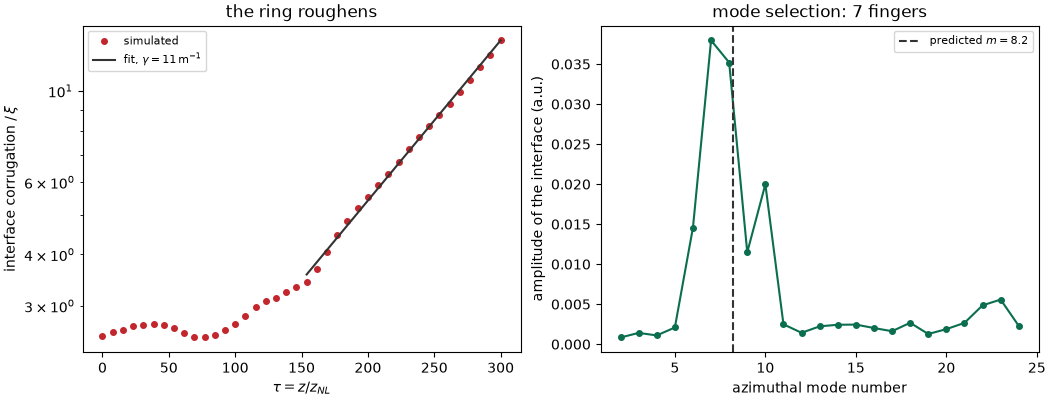
mode selected 7, predicted 8.2
measured growth 10.8 /m against 15.9 predicted

Three planes

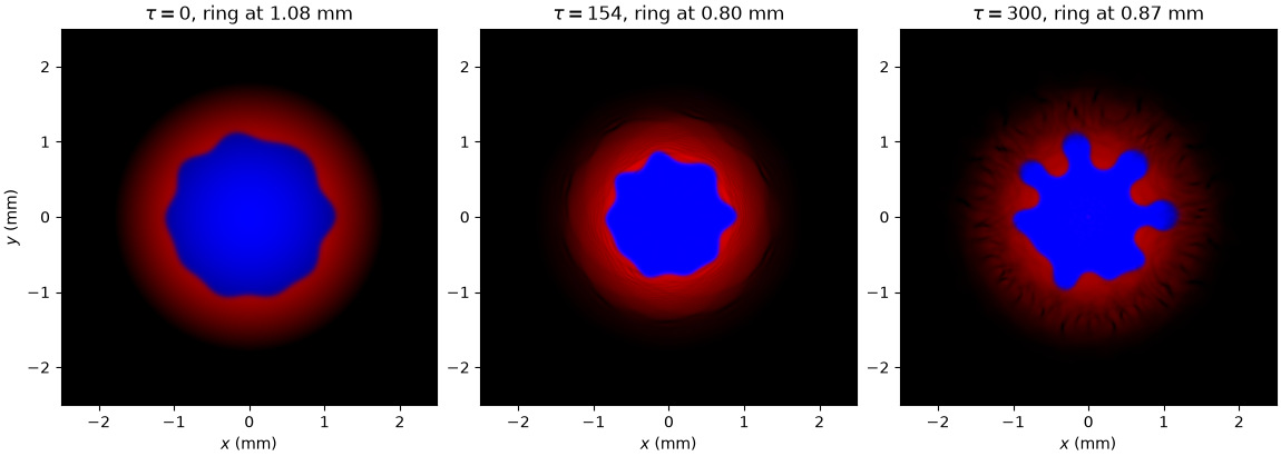
Dense component in red, light in blue: the seeded ring, the fingers growing, and the rounded caps that make a Rayleigh-Taylor mushroom. The shell sinks as it goes, which is the potential energy the instability is spending.

def composite(pair):
    """Return an RGB image with the dense fluid red and the light one blue."""
    dense, light = pair
    rgb = np.zeros((*dense.shape, 3))
    rgb[..., 0] = np.clip(dense / I_PEAK, 0, 1)
    rgb[..., 2] = np.clip(light / (I_PEAK / 3), 0, 1)
    return rgb


EXTENT = [simu.X[0] * 1e3, simu.X[-1] * 1e3, simu.Y[0] * 1e3, simu.Y[-1] * 1e3]
fig, axes = plt.subplots(1, 3, figsize=(11.5, 4.1), layout="constrained")
for ax, frame in zip(axes, (0, len(frames) // 2, len(frames) - 1)):
    ax.imshow(composite(frames[frame]), origin="lower", extent=EXTENT)
    radius = np.nanmean(interface_radius(*frames[frame]))
    ax.set_title(rf"$\tau = {taus[frame]:.0f}$, ring at {radius * 1e3:.2f} mm")
    ax.set_xlabel("$x$ (mm)")
axes[0].set_ylabel("$y$ (mm)")
plt.show()

The whole propagation

fig, ax = plt.subplots(figsize=(5.2, 5.2), layout="constrained")
picture = ax.imshow(composite(frames[0]), origin="lower", extent=EXTENT)
ax.set_xlabel("$x$ (mm)"), ax.set_ylabel("$y$ (mm)")


def show(frame):
    """Draw one sampled plane."""
    picture.set_data(composite(frames[frame]))
    ax.set_title(rf"$\tau = {taus[frame]:.0f}$")
    return (picture,)


# Bound at module level rather than dropped: sphinx-gallery looks through the
# example's namespace for an Animation and embeds what it finds there, so one
# that only exists inside a function is a still picture on the page.
anim = FuncAnimation(fig, show, frames=len(frames), interval=110, blit=False)
plt.show()